Running spatial machine learning models

The default MBG setup models a uniform linear relationship between each covariate and the outcome in modeling space. This assumption may not always hold: there may be nonlinear relationships, spatially-varying relationships, and covariate interactions that affect the outcome. If we want to capture the nuances of these predictor relationships without over-fitting our model, we can turn to machine learning (ML) algorithms that are intended to fit over a high-dimensional feature space.

Setup

In this tutorial, we will run multiple machine learning models using point-georeferenced outcome data and raster covariate data, then apply the ML model predictions to generate raster predictions across the prediction space. To begin, load the mbg package and helper packages for data manipulation, then load the example data. Generate a raster of the full prediction space using the build_id_raster() function.

## Load packages
library(data.table)
library(sf)
library(terra)
library(mbg)

## Load data
# Outcome: child stunting
outcomes <- data.table::fread(
  system.file('extdata/child_stunting.csv', package = 'mbg')
)
# Spatial covariates, including an intercept
covariates <- list(
  access = terra::rast(system.file('extdata/access.tif', package = 'mbg')),
  evi = terra::rast(system.file('extdata/evi.tif', package = 'mbg')),
  temperature = terra::rast(system.file('extdata/temperature.tif', package = 'mbg'))
)
covariates$intercept <- covariates[[1]] * 0 + 1
# Administrative boundaries
# Departments (first-level administrative divisions)
departments <- sf::st_read(
  system.file('extdata/Benin_departments.gpkg', package = 'mbg'),
  quiet = TRUE
)

# Create ID raster
id_raster <- mbg::build_id_raster(
  polygons = departments,
  template_raster = covariates[[1]]
)

Running ML models with mbg and caret

The mbg package wraps the caret package to run predictive models over space. The caret (Classification And REgression Training) package contains 137 different model specifications for regression: these include linear regression and generalized linear models, generalized additive models, penalized regression (LASSO, ridge, elastic net), support vector machines, regression trees, gradient boosting, neural nets, and more.

You can search the full list of available regression models in the caret documentation. Note that some models have tuning parameters that can be set beforehand. We will create a named list of submodel_settings, where each name corresponds to the name of the model we will be using, and each value is an optional named list containing any tuning parameters we want to pass to that model.

Each ML model will be tuned using cross-validation. We can control model tuning by editing cross_validation_settings, a named list of arguments that will be passed to the caret::trainControl function.

These models are fit and predictions generated across the study area using the run_regression_submodels() function. This function returns a named list with two items:

• "models": The fitted caret models, which can be used to closely inspect the model results and generate new predictions
• "predictions": Rasters containing the predictions of the outcome generated from each model.

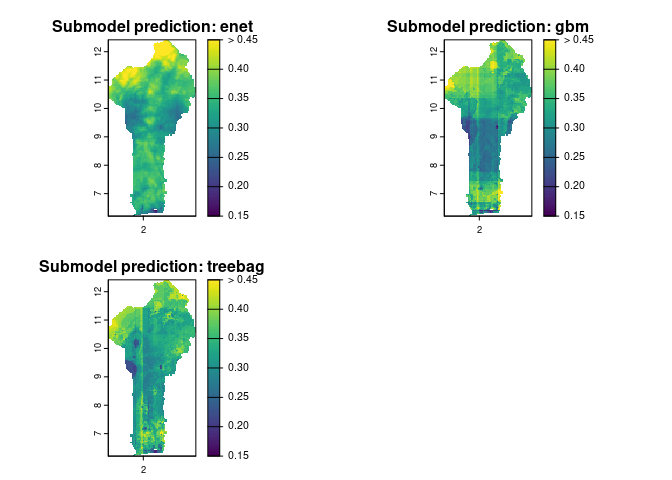
In the code block below, we run three regression models, using child stunting in Benin as the outcome and three covariate predictors: elastic net (a penalized regression method), gradient boosted machines, and bagged regression trees. We then plot the results across Benin:

## Run ML models using input covariates
cross_validation_settings <- list(method = 'repeatedcv', number = 5, repeats = 5)
submodel_settings <- list(
  enet = NULL,
  gbm = list(verbose = FALSE),
  treebag = NULL
)
submodels <- mbg::run_regression_submodels(
  input_data = outcomes,
  id_raster = id_raster,
  covariates = covariates,
  cv_settings = cross_validation_settings,
  model_settings = submodel_settings,
  prediction_range = c(0, 1)
)
#> Fitting 3 regression models
#>   Candidate model:  enet
#> Loading required package: ggplot2
#> Loading required package: lattice
#>   Candidate model:  enet: 0.932 sec elapsed
#>   Candidate model:  gbm
#>   Candidate model:  gbm: 1.825 sec elapsed
#>   Candidate model:  treebag
#>   Candidate model:  treebag: 2.508 sec elapsed
#> Fitting 3 regression models: 5.377 sec elapsed

plot(
  terra::rast(submodels$predictions),
  main = paste('Submodel prediction:', names(submodels$predictions)),
  range = c(.15, .45),
  fill_range = TRUE
)

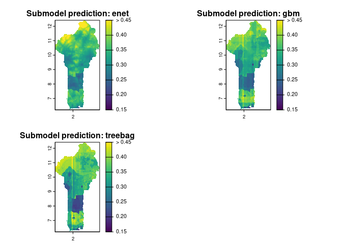
Many machine learning models are robust to handling a large feature space, meaning that we can add more candidate predictors to the model without over-fitting. The run_regression_submodels() includes the option to add administrative boundaries to the feature space as one-hot encoded variables. In the code block below, we use this option to add department (first-level administrative division) identifiers to the predictors:

submodels_with_department_effects <- mbg::run_regression_submodels(
  input_data = outcomes,
  id_raster = id_raster,
  covariates = covariates,
  cv_settings = cross_validation_settings,
  model_settings = submodel_settings,
  use_admin_bounds = TRUE,
  admin_bounds = departments,
  admin_bounds_id = 'department_code',
  prediction_range = c(0, 1)
)
#> Fitting 3 regression models
#>   Candidate model:  enet
#>   Candidate model:  enet: 1.055 sec elapsed
#>   Candidate model:  gbm
#>   Candidate model:  gbm: 2.548 sec elapsed
#>   Candidate model:  treebag
#>   Candidate model:  treebag: 3.82 sec elapsed
#> Fitting 3 regression models: 7.529 sec elapsed

plot(
  terra::rast(submodels_with_department_effects$predictions),
  main = paste('Submodel prediction:', names(submodels_with_department_effects$predictions)),
  range = c(.15, .45),
  fill_range = TRUE
)

Stacking ML models

The run_regression_submodels() function allows users to estimate the outcome based on many different types of regression models which may not make similar predictions across the study area. How can we combine estimates from these models while also incorporating some of the geostatistical principles used in the baseline mbg model? One option is to use stacked generalization, which combines model predictions to create a “super learner” with better performance than any individual model. Previous studies indicate that this “super learner” ensemble can replace the covariate term in a standard geostatistical model to improve prediction accuracy.

To run a geostatistical model with stacked generalization, create a MbgModelRunner object where use_stacking = TRUE. The arguments submodel_settings, stacking_cv_settings, and stacking_prediction_range should also be set when running stacked generalization. In the example below, we also include administrative effects as one-hot encoded variables in the component submodels.

After enabling stacking, run the MbgModelRunner$run_mbg_pipeline() method to complete the full model workflow. This will now include the following steps:

• Run the component regression submodels
• For each submodel, create estimates of the outcome at each pixel across the study area
• Run the geostatistical model, replacing the standard covariate effect with the “super learner” ensemble based on the regression submodels
• Generate final predictions from the geostatistical model

# Run stacked generalization MBG model
model_runner <- MbgModelRunner$new(
  input_data = outcomes,
  id_raster = id_raster,
  covariate_rasters = covariates,
  use_stacking = TRUE,
  stacking_cv_settings = cross_validation_settings,
  stacking_model_settings = submodel_settings,
  stacking_prediction_range = c(0, 1),
  stacking_use_admin_bounds = TRUE,
  admin_bounds = departments,
  admin_bounds_id = 'department_code'
)
model_runner$run_mbg_pipeline()
#> Fitting 3 regression models
#>   Candidate model:  enet
#>   Candidate model:  enet: 1.219 sec elapsed
#>   Candidate model:  gbm
#>   Candidate model:  gbm: 2.403 sec elapsed
#>   Candidate model:  treebag
#>   Candidate model:  treebag: 3.434 sec elapsed
#> Fitting 3 regression models: 7.2 sec elapsed
#> MBG model fitting
#> MBG model fitting: 12.556 sec elapsed
#> Generating model predictions
#>   Parameter posterior samples
#>   Parameter posterior samples: 5.23 sec elapsed
#>   Cell draws
#>   Cell draws: 2.128 sec elapsed
#>   Summarize draws
#>   Summarize draws: 1.447 sec elapsed
#> Generating model predictions: 8.807 sec elapsed

When use_stacking = TRUE, the submodel predictions are saved in the MbgModelRunner$model_covariates attribute. These can be pulled and plotted:

# Get predictions from each component submodel
mbg_component_models <- model_runner$model_covariates

plot(
  terra::rast(model_runner$model_covariates),
  range = c(.15, .45),
  fill_range = TRUE
)

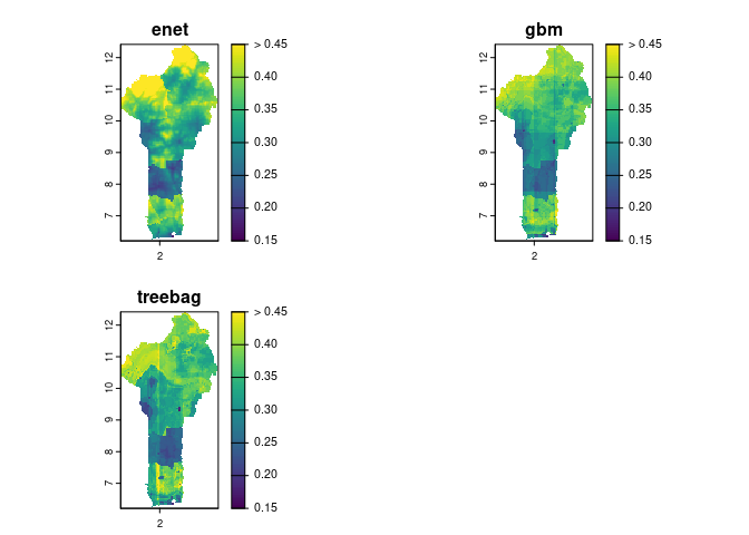
We can also plot mean estimates from the geostatistical model. Note how the geostatistical model blends estimates from the component submodels, while also including other effects including the latent spatial term and the nugget:

# Get predictions from the overall model
grid_cell_predictions <- model_runner$grid_cell_predictions
# Plot mean estimates
plot(
  grid_cell_predictions$cell_pred_mean,
  main = 'MBG mean estimates'
)
lines(departments)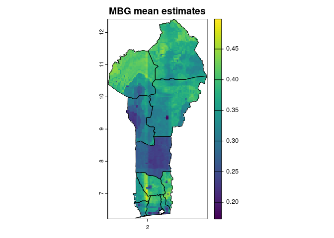

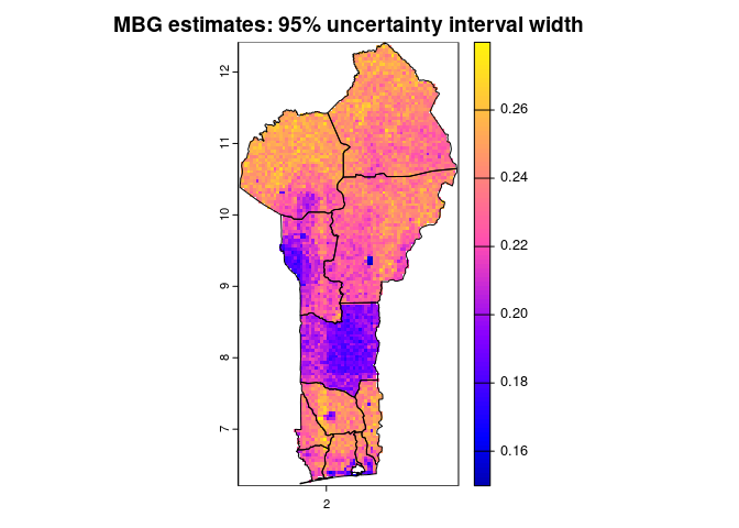
As as with the default model, we can plot uncertainty by pixel:

ui_raster <- grid_cell_predictions$cell_pred_upper - grid_cell_predictions$cell_pred_lower
plot(
  ui_raster,
  col = sf::sf.colors(n = 100),
  main = 'MBG estimates: 95% uncertainty interval width'
)
lines(departments)